Acoustic Feature Demo
[1]:
import avn.dataloading as dataloading
import avn.acoustics as acoustics

import pandas as pd
In this tutorial, we will be using the avn.acoustics module to calculate a suite of acoustic features first for a single period of song, then for all syllables in a syllable table. The song features included in avn are based on those in Sound Analysis Pro (SAP). They include: - Goodness of Pitch - Mean Frequency - Wiener Entropy - Amplitude - Amplitude Modulation - Frequency Modulation - Pitch
I plan to add a notebook with more information about each of these features in the future, but in the meantime more detailed descriptions of the features can be found in the Sound Analysis Pro documentation here: http://soundanalysispro.com/manual/chapter-4-the-song-features-of-sap2
Calculating Acoustic Features for a Single Song Interval
Creating a SongInterval Object
AVN’s acoustics module centers around a class called SongInterval. This class stores information about a particular interval of audio, be that a song motif, a single syllable, or a full .wav file. It also has many methods which allow you to quickly calculate each acoustic feature across the interval and to extract summary statistics for each feature.
Let’s begin by loading an example .wav file using AVN’s dataloading module:
[2]:
song = dataloading.SongFile("../sample_data/G402/G402_43362.23322048_9_19_6_28_42.wav")
We create our SongInterval object by passing this SongFile type object as an input to acoustics.SongInterval(). You also have the option to pass the onset and offset timestamps within the file of your interval of interest, but if these aren’t specified the SongInterval will consist of the full file. In this tutorial, we will be looking at only the first 2 seconds of the file.
[3]:
song_interval = acoustics.SongInterval(song, onset = 0, offset = 2)
acoustics.SongInterval() also has many other optional parameters that you can set to change how the acoustic features are calculated. The default parameters are well suited for the analysis of zebra finch song and match those used by Sound Analysis Pro. It is unlikely that you would have need to change them, but if you’re curious the full list of parameters, their default values, and a brief explanation of how each is used is available in the docstring of the SongInterval class.
Calculating Acoustic Features
Now that we have our SongInterval object ready, we can calculate any single acoustic feature over this interval by calling one of the following functions:
.calc_goodness()to calculate the goodness of pitch.calc_mean_frequency()to calculate the mean frequency.calc_frequency_modulation()to calculate the frequency modulation.calc_amplitude_modulation()to calculate the amplitude modulation.calc_entropy()to calculate the Weiner entropy.calc_amplitude()to calculate the amplitude.calc_pitch()to estimate the fundamental frequency
Each of these functions will return a numpy array containing the value of the acoustic feature for each short time window in the song interval. As an example, let’s calculate the goodness of pitch.
[4]:
goodness = song_interval.calc_goodness()
print("Shape of Output: " + str(goodness.shape))
goodness
Shape of Output: (2206,)
[4]:
array([0.08748554, 0.08418637, 0.08150075, ..., 0.07466519, 0.09283684,
       0.08723036])
If you want to calculate multiple acoustic features, this can be done more efficiently with the .calc_all_features() method. You can pass this method a list of all the acoustic features that you want to calculate and it will return them as a dictionary. By default, all available acoustic features will be returned but if you don’t need all of them you can pass a list of only those features that you do want as the features parameter. For this to work, the names of the features must be
spelled correctly, with the correct capitalization. That is: [‘Goodness’, ‘Mean_frequency’, ‘Frequency_modulation’, ‘Amplitude_modulation’, ‘Amplitude’, ‘Entropy’, ‘Pitch’].
Let’s calculate just the goodness of pitch and the amplitude in this example:
[5]:
features = song_interval.calc_all_features(features = ['Goodness', 'Amplitude'])
features
[5]:
{'Goodness': array([0.08748554, 0.08418637, 0.08150075, ..., 0.07466519, 0.09283684,
        0.08723036]),
 'Amplitude': array([44.05477002, 45.21658021, 46.0164633 , ..., 47.51012431,
        46.92642835, 46.14961101])}
Visualizing Acoustic Features
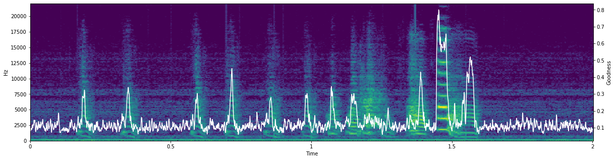
SongInterval also has a handy plotting function which can plot any acoustic feature over a spectrogram of the interval. Let’s have a look at some of those features:
[6]:
song_interval.plot_feature(feature = "Goodness")
<Figure size 1440x360 with 0 Axes>
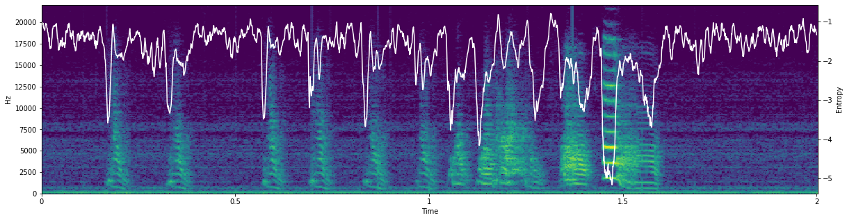
[7]:
song_interval.plot_feature(feature = "Entropy")
<Figure size 1440x360 with 0 Axes>
This will work for any of the acoustic features in avn.acoustics (‘Goodness’, ‘Mean_frequency’, ‘Frequency_modulation’, ‘Amplitude_modulation’, ‘Amplitude’, ‘Entropy’, or ‘Pitch’)
Calculating Acoustic Feature Summary Statistics
Now we know how to calculate acoustic features for each frame in a song interval. These can be interesting if you are curious about how a feature changes over the course of a syllable, for example, but it is generally more useful to have a single score per feature per interval. Thankfully, SongInterval also has a method to calculate summary statistics for each acoustic feature over the interval. Let’s do that for all the features available (which is the default if we don’t specify a subset
of features) by calling .calc_feature_stats().
[8]:
feature_stats = song_interval.calc_feature_stats()
feature_stats
[8]:
| Goodness | Mean_frequency | Entropy | Amplitude | Amplitude_modulation | Frequency_modulation | Pitch | |
|---|---|---|---|---|---|---|---|
| mean | 0.137592 | 2891.814561 | -1.803505 | 56.846695 | 0.000021 | 0.454302 | 3511.723555 |
| std | 0.091330 | 747.591179 | 0.696087 | 11.296620 | 0.399036 | 0.354409 | 2397.807850 |
| min | 0.059758 | 1417.312546 | -5.164130 | 44.054770 | -4.353593 | 0.001553 | 538.585520 |
| 25% | 0.096266 | 2385.826963 | -2.058598 | 47.804789 | -0.011437 | 0.156986 | 1133.268704 |
| 50% | 0.112000 | 2833.490716 | -1.590509 | 49.840404 | -0.000314 | 0.388846 | 4277.993715 |
| 75% | 0.135132 | 3322.131753 | -1.339322 | 66.323051 | 0.008567 | 0.695680 | 5967.726910 |
| max | 0.799963 | 5229.989962 | -0.792397 | 90.562486 | 4.662347 | 1.565718 | 7297.810765 |
It is a bit silly to calculate these features over such a long interval as in this example, but these scores can be very valuable when calculated over single syllables. They can be used to cluster syllables, to detect unusual syllable types, to measure the variability of individual syllable types, or to detect changes in song structure before and after a manipulation, etc.
Saving Features
SongInterval also has built in functions to save acoustic features or acoustic feature statistics .csv files. You can save the full time series of features with the method .save_features(), which takes as input out_file_path (the path to the folder where you want to save the features), file_name (the root name you want to give the file), and features(the list of features you want to save - if unspecified all will be saved). This will save a file called
file_name_features.csv in the designated output folder, as well as a file called file_name_metadata.csv which contains all the parameter values used to calculate the features, as well as the avn version, the original file name and the onset and offset timestamps of the interval within the file. This metadata information will ensure that your acoustic feature calculations will be reproducible in the future.
[9]:
song_interval.save_features(out_file_path="../sample_data/", file_name = "G402_sample_song")
You can also save the summary statistics in exactly the same way with the method save_feature_stats(). The output files will be called file_name_feature_stats.csv and file_name_metadata.csv.
[10]:
song_interval.save_feature_stats(out_file_path="../sample_data/", file_name = "G402_sample_song")
Calculate Acoustic Features for Many Syllables
In the first section of this tutorial we outlined how to use the avn.acoustics module to calculate acoustic features for a single interval of audio. However, a more common workflow is to calculate the acoustic features for many syllables at a time so that they can be compared, clustered etc. Thankfully, the avn.acoustics module also has a dedicated class to make it easier to handle large tables of song syllables!
Creating an AcousticData Object
Similarly to the avn.syntax.SyntaxData class, the avn.acoustics module has an AcousticData class which stores a table of syllables, and has convenient methods to calculate the acoustic features of each of those syllables.
To begin, we need a table with one row for every syllable that we want to analyze. This table should have the following columns: - files which should contain the name of the .wav file in which the syllable is found - onsets which should contain the onset timestamp of the syllable in seconds within the file - offsets which should contain the offset timestamp of the syllable in seconds within the file.
Such a table can be generated using the avn.segmentation module, or whatever your preferred syllable segmentation method is as long as it has columns structured as described above.
The syllable table can also contain any number of other columns (such as syllable labels, notes, etc.) which will be preserved but are not necessary.
Here is an example of what such a syllable table could look like:
[11]:
syll_df = pd.read_csv("../sample_data/G402_syll_df.csv")
syll_df
[11]:
| files | onsets | offsets | labels | |
|---|---|---|---|---|
| 0 | G402_43362.23322048_9_19_6_28_42.wav | 0.166009 | 0.225170 | i |
| 1 | G402_43362.23322048_9_19_6_28_42.wav | 0.321043 | 0.385828 | i |
| 2 | G402_43362.23322048_9_19_6_28_42.wav | 0.570295 | 0.626757 | i |
| 3 | G402_43362.23322048_9_19_6_28_42.wav | 0.690363 | 0.751837 | i |
| 4 | G402_43362.23322048_9_19_6_28_42.wav | 0.828390 | 0.898912 | i |
| ... | ... | ... | ... | ... |
| 589 | G402_43362.43586086_9_19_12_6_26.wav | 1.808186 | 1.976712 | b |
| 590 | G402_43362.43586086_9_19_12_6_26.wav | 2.011905 | 2.095646 | c |
| 591 | G402_43362.43586086_9_19_12_6_26.wav | 2.114762 | 2.263175 | d |
| 592 | G402_43362.43586086_9_19_12_6_26.wav | 2.318934 | 2.402177 | e |
| 593 | G402_43362.43586086_9_19_12_6_26.wav | 2.433810 | 2.563447 | f |
594 rows × 4 columns
We can create a new AcousticData object by passing this syllable table as input to acoustics.AcousticData(), along with the Bird_ID of the subject bird and the path to the folder containing the .wav files in the syllable table. Like so:
[12]:
acoustic_data = acoustics.AcousticData(Bird_ID = "G402", syll_df = syll_df, song_folder_path="../sample_data/G402/")
Calculate Acoustic Features
We can now calculate any combination of acoustic features from this list: [‘Goodness’, ‘Mean_frequency’, ‘Frequency_modulation’, ‘Amplitude_modulation’, ‘Amplitude’, ‘Entropy’, ‘Pitch’] for each syllable in the syllable table with the method .calc_all_features().
For example, let’s calculate the Frequency modulation and the Pitch:
[13]:
features = acoustic_data.calc_all_features(features = ['Pitch', 'Frequency_modulation'])
features
[13]:
| Frequency_modulation | Pitch | files | onsets | offsets | labels | |
|---|---|---|---|---|---|---|
| 0 | [1.554138752062315, 1.522665756024348, 1.39044... | [1342.9870358953176, 1343.6980823646277, 1347.... | G402_43362.23322048_9_19_6_28_42.wav | 0.166009 | 0.22517 | i |
| 0 | [1.1951050687546656, 1.2754715619300896, 1.390... | [1337.81447860608, 1340.4311096227414, 1344.11... | G402_43362.23322048_9_19_6_28_42.wav | 0.321043 | 0.385828 | i |
| 0 | [1.5256539450074136, 1.4687677891619524, 1.055... | [1334.094750632218, 1332.705804681969, 1337.61... | G402_43362.23322048_9_19_6_28_42.wav | 0.570295 | 0.626757 | i |
| 0 | [1.2974545304143592, 1.1919562335359768, 0.876... | [1379.7435850832105, 1394.0666879679236, 1405.... | G402_43362.23322048_9_19_6_28_42.wav | 0.690363 | 0.751837 | i |
| 0 | [1.4339299730529087, 0.9783459018679432, 0.460... | [1341.9634801933178, 1357.344164568718, 1365.5... | G402_43362.23322048_9_19_6_28_42.wav | 0.82839 | 0.898912 | i |
| ... | ... | ... | ... | ... | ... | ... |
| 0 | [1.175703506965015, 1.0612232718381467, 0.9003... | [4838.566260423787, 4807.5771214231645, 4803.9... | G402_43362.43586086_9_19_12_6_26.wav | 1.808186 | 1.976712 | b |
| 0 | [1.5624430371801388, 1.5534304047914287, 0.858... | [4059.867476677284, 4130.549387945176, 4148.93... | G402_43362.43586086_9_19_12_6_26.wav | 2.011905 | 2.095646 | c |
| 0 | [1.3678523064969446, 1.3134255155920922, 1.232... | [1808.7585386523256, 1808.5561471447486, 1809.... | G402_43362.43586086_9_19_12_6_26.wav | 2.114762 | 2.263175 | d |
| 0 | [1.3641694039563599, 1.325291611030776, 1.2633... | [568.0846693657795, 567.4237886580611, 566.769... | G402_43362.43586086_9_19_12_6_26.wav | 2.318934 | 2.402177 | e |
| 0 | [1.5496912993782248, 1.5060051496775306, 1.328... | [3933.414997549934, 3942.7519148349297, 3918.4... | G402_43362.43586086_9_19_12_6_26.wav | 2.43381 | 2.563447 | f |
594 rows × 6 columns
As you can see, this method returns a new dataframe with all the columns in our original syllable table, plus a column for each acoustic feature we specified where each row contains a numpy array with the value of the feature at every short time window within each syllable. This table will also be saved as an attribute of acoustic_data called all_features.
[16]:
acoustic_data.all_features.head()
[16]:
| Frequency_modulation | Pitch | files | onsets | offsets | labels | |
|---|---|---|---|---|---|---|
| 0 | [1.554138752062315, 1.522665756024348, 1.39044... | [1342.9870358953176, 1343.6980823646277, 1347.... | G402_43362.23322048_9_19_6_28_42.wav | 0.166009 | 0.22517 | i |
| 0 | [1.1951050687546656, 1.2754715619300896, 1.390... | [1337.81447860608, 1340.4311096227414, 1344.11... | G402_43362.23322048_9_19_6_28_42.wav | 0.321043 | 0.385828 | i |
| 0 | [1.5256539450074136, 1.4687677891619524, 1.055... | [1334.094750632218, 1332.705804681969, 1337.61... | G402_43362.23322048_9_19_6_28_42.wav | 0.570295 | 0.626757 | i |
| 0 | [1.2974545304143592, 1.1919562335359768, 0.876... | [1379.7435850832105, 1394.0666879679236, 1405.... | G402_43362.23322048_9_19_6_28_42.wav | 0.690363 | 0.751837 | i |
| 0 | [1.4339299730529087, 0.9783459018679432, 0.460... | [1341.9634801933178, 1357.344164568718, 1365.5... | G402_43362.23322048_9_19_6_28_42.wav | 0.82839 | 0.898912 | i |
Calculate Acoustic Feature Summary Statistics
As mentioned in the first section of this tutorial, it is often more useful to have a single mean and std value for each feature for each syllable, instead of time series (which will take more disk space to save and are all different lengths for different syllables making them difficult to work with). To get just the summary statistics for the acoustic features for each syllable in the acoustic_data syllable table, we can use the method .calc_all_feature_stats().
Let’s calculate the summary statistics for the mean frequency for every syllable in our table:
[22]:
feature_stats = acoustic_data.calc_all_feature_stats(features = ['Mean_frequency'])
feature_stats
[22]:
| Syll_info | Mean_frequency | ||||||||||
|---|---|---|---|---|---|---|---|---|---|---|---|
| files | onsets | offsets | labels | mean | std | min | 25% | 50% | 75% | max | |
| 0 | G402_43362.23322048_9_19_6_28_42.wav | 0.166009 | 0.22517 | i | 2907.785023 | 1121.457694 | 1412.581905 | 2144.890471 | 2500.659910 | 3946.849894 | 4906.114381 |
| 1 | G402_43362.23322048_9_19_6_28_42.wav | 0.321043 | 0.385828 | i | 2703.070150 | 941.459831 | 1498.764199 | 1765.620166 | 2566.293475 | 3330.237660 | 4636.205351 |
| 2 | G402_43362.23322048_9_19_6_28_42.wav | 0.570295 | 0.626757 | i | 3012.216848 | 1175.352043 | 1562.812118 | 2162.649309 | 2471.829333 | 4066.341596 | 5047.588192 |
| 3 | G402_43362.23322048_9_19_6_28_42.wav | 0.690363 | 0.751837 | i | 2916.965205 | 1049.030479 | 1504.505563 | 2223.822274 | 2500.249679 | 3732.941696 | 4843.951932 |
| 4 | G402_43362.23322048_9_19_6_28_42.wav | 0.82839 | 0.898912 | i | 2724.163727 | 944.713327 | 1504.298356 | 1965.995565 | 2532.514305 | 3406.932164 | 4577.235024 |
| ... | ... | ... | ... | ... | ... | ... | ... | ... | ... | ... | ... |
| 589 | G402_43362.43586086_9_19_12_6_26.wav | 1.808186 | 1.976712 | b | 4211.076484 | 930.050590 | 1923.876639 | 3771.950718 | 4486.205261 | 4859.350242 | 5467.731391 |
| 590 | G402_43362.43586086_9_19_12_6_26.wav | 2.011905 | 2.095646 | c | 3909.581357 | 326.175365 | 3197.165752 | 3650.098384 | 3947.938012 | 4124.447948 | 4458.822812 |
| 591 | G402_43362.43586086_9_19_12_6_26.wav | 2.114762 | 2.263175 | d | 3771.857709 | 348.871318 | 3010.147580 | 3600.451037 | 3732.176595 | 3915.852528 | 5122.593444 |
| 592 | G402_43362.43586086_9_19_12_6_26.wav | 2.318934 | 2.402177 | e | 3997.790057 | 272.362455 | 3387.536710 | 3781.849900 | 4105.547617 | 4231.509360 | 4317.167893 |
| 593 | G402_43362.43586086_9_19_12_6_26.wav | 2.43381 | 2.563447 | f | 3770.705568 | 554.947440 | 1941.667383 | 3547.984968 | 3958.680979 | 4109.973595 | 4351.028939 |
594 rows × 11 columns
Saving Features
Like the SongInterval class, the AcousticData class also has methods to automatically save your acoustic features, along with a metadata file with all the information necessary to reproduce their calculation.
While it is possible to save the timeseries of each acoustic feature for every syllable with the method .save_features(), this will occupy considerable disk space and usually isn’t necessary. Instead, I suggest saving just the summary statistics for each feature with the method .save_feature_stats().
Both .save_features() and .save_feature_stats() take as input an out_file_path (the path to the folder where you want the .csv files to be saved), file_name (the root name you want to give the file) and features (the list of features you want to save. If this is not specified all features will be saved).
Let’s save the summary statistics for Goodness of Pitch and Amplitude for all the syllables in our table:
[23]:
acoustic_data.save_feature_stats(out_file_path="../sample_data/", file_name = "G402_syll_table", features = ["Goodness", "Amplitude"])
This calculates and saves the summary statistics for each acoustic feature specified in a file called G402_syll_table_all_feature_stats.csv, and saves a file called G402_syll_table_metadata.csv.